
As part of the initial studying for my final year project (more on that in a future blog post), I had to learn how to build deep models for text classification. As a newbie to deep learning at the time, I decided to start with a small project to familiarize myself with deep learning concepts, TensorFlow and the field of text classification. After some digging, I decided to build classifiers for the movie review sentence polarity dataset (Pang and Lee, 2004) since this was a relatively smaller dataset, dealt with sentences (as opposed to documents) and was a binary classification task. Additionally, there were multiple existing references that I could use as a starting point, which proved to be extremely useful. The complete source code and detailed results for my project can be found on GitHub.
There were three main models I built for the classification task — a convolutional neural network that processed each sentence with words replaced by word embeddings (Model v1, based on Yoon Kim’s 2014 paper), a convolutional neural network that processed each sentence with words replaced by similarity vectors calculated from word embeddings (Model v2) and a graph convolutional neural network that processed each sentence as a TF-IDF vector with the feature graph constructed from word embeddings (Model v3, based on M. Defferrard’s 2016 paper). All three networks used Google’s word2vec (Google Code Archive) as pre-trained word embeddings.
Model v1 - Convolutional Neural Network
This model consists of an embedding layer followed by multiple parallel convolutional + max-pool layers before the outputs are combined and classified by a softmax layer.
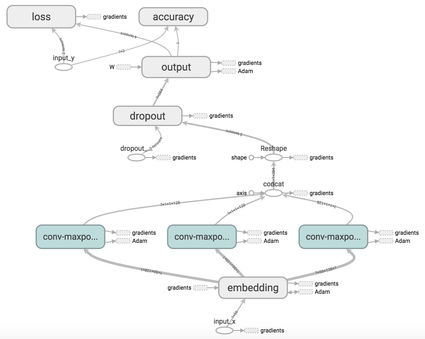
Computational Graph for Model v1
Training 128-dimensional word embeddings from scratch along with the network resulted in a model with a maximum test accuracy of 74.30%, however, training the model with the pre-trained 300-dimensional embeddings from Google resulted in a maximum test accuracy of 79.46%. An interesting point to note was that fine-tuning the embeddings for the task at hand (as opposed to keeping them static) consistently resulted in a slight bump in accuracy (and allowed to model to completely converge).
Model v2 - CNN on Similarity Vectors
While building and training Model v1 with different hyperparameters, I explored the resulting embeddings in terms of the cosine distance between certain words. For example, the words “good” & “bad” were very similar in the embeddings provided by Google (perhaps due to their syntactic purpose) but the network learned to treat them on opposite ends of the spectrum considering the task at hand.
Thus, I decided to feed the model the cosine distances between words directly by using the same architecture as Model v1 but replacing the 300-dimensional word embeddings with 18,758-dimensional vectors that contained the cosine distances to every other word in the vocabulary (calculated from the word embeddings). This is obviously not a practical model but it allowed me to experiment with representing the vocabulary as a “graph” where each 18,758-dimensional vector represented the edge weights of a word (i.e. node) to every other word (i.e. node) in the vocabulary.
The resulting model had a lot of trainable parameters (and took a very long time to train) but had a maximum test accuracy of 75.61% (lower than Model v1).
Model v3 - Graph Convolutional Neural Network
I wanted to take the idea of representing the vocabulary as a graph further and decided to implement a graph convolutional neural network for the classification problem. The feature graph is a 16-NN graph constructed from the pre-trained word embeddings of the 5,000 most frequent words in the vocabulary and each sentence is represented by its TF-IDF vector (using scikit-learn’s TfidfVectorizer). The model runs the sentence through graph convolutional + pooling layer(s) sequentially followed by an output softmax layer.
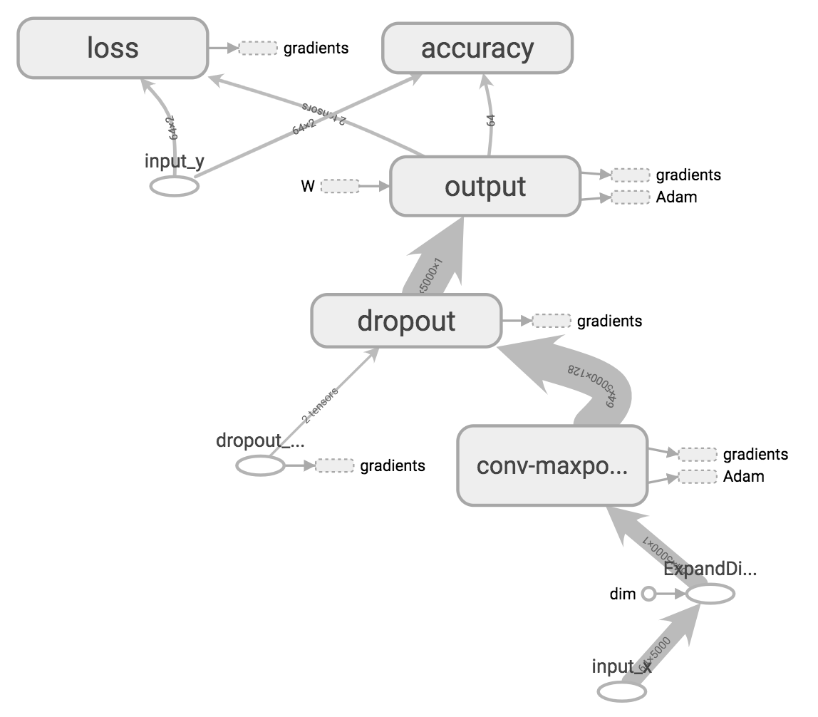
Computational Graph for Model v3
The model had a maximum test accuracy of 76.17% with a single graph convolutional layer and did not have a significant increase in performance with additional graph convolutional layers.
Summary
| Model | Test Accuracy |
|---|---|
| Multinomial Naive Bayes (TF-IDF Vectors) | 77.58% |
| Model v1 (CNN) | 74.30% |
| Model v1.2 (CNN w/ Pre-Trained Embeddings) | 79.46% |
| Model v2 (CNN on Similarity Vectors) | 75.61% |
| Model v3 (Graph CNN) | 76.17% |
Overall, most of the models I implemented tend to hover around 75% - 79% test accuracy for the movie review dataset with multiple trials, which is only slightly better than the Multinomial Naive Bayes benchmark (which takes a significantly less amount of time to train).
In closing, while the results of my project aren’t groundbreaking, implementing all the models and learning the concepts behind them was very educational and serves as a great foundation for my final year project!